Recover the data via GovData

The data is accessible via govdata.de an easy way to get, use and share data about Germany. If you don’t speak German I’d suggest you use the curl package to download the data directly from the website.

# Some settings
temp <- tempfile()
url <- "https://www.bundeswahlleiter.de/dam/jcr/72f186bb-aa56-47d3-b24c-6a46f5de22d0/btw17_kerg.csv"

# Then download it
curl_download(url, temp)

# And read it
bundeswahl <- read.csv2(temp, skip = 5)

I use read.csv2() because of the European .csv format (alternatively, you can add an argument sep = ';') and skip two rows of useless information. Afterwards, a quick look at the first rows shows us this.

head(bundeswahl[, 1:10])
##   Nr                            Gebiet gehört.zu Wahlberechtigte
## 1 NA                                          NA     Erststimmen
## 2 NA                                          NA       Endgültig
## 3  1             Flensburg – Schleswig         1          228471
## 4  2 Nordfriesland – Dithmarschen Nord         1          186568
## 5  3      Steinburg – Dithmarschen Süd         1          176636
## 6  4             Rendsburg-Eckernförde         1          200831
##            X          X.1        X.2      Wähler        X.3          X.4
## 1            Zweitstimmen            Erststimmen            Zweitstimmen
## 2 Vorperiode    Endgültig Vorperiode   Endgültig Vorperiode    Endgültig
## 3     226944       228471     226944      171914     162749       171914
## 4     186177       186568     186177      139194     131527       139194
## 5     176731       176636     176731      132017     126409       132017
## 6     198903       200831     198903      157354     149583       157354

The two first rows are going to be problematic as all underlying numbers are read as factor. To quickly circumvent this issue and as this information is highly repetitive, I propose that we save the column names and read the data again skipping two more rows.

# Save names
coldim <- colnames(bundeswahl)

# Read again and rename columns
bundeswahl <- read.csv2(temp, skip = 7)
colnames(bundeswahl) <- coldim

We’re all set! What we need is a convenient way to pull apart information about each vote. If you remember that the first two columns are always first vote (this year’s election and 2013) whereas the second two columns are always second vote, it isn’t really challenging.

To get this year’s first suffrage via column names simply use grep() and grab columns with real information.

# Find this year's first suffrage column's number
vot1new <- grep("X", coldim, invert = TRUE)

Other vote results can be easily deduced but don’t forget that the three first columns are always the same.

vot1old <- c(vot1new[1:3], sapply(vot1new[4:length(vot1new)], function(x) x+1))
vot2new <- c(vot1new[1:3], sapply(vot1new[4:length(vot1new)], function(x) x+2))
vot2old <- c(vot1new[1:3], sapply(vot1new[4:length(vot1new)], function(x) x+3))

Last thing, we need to isolate cities and states, which are both in this .csv. The column gehört.zu contains this information. Numbers vary from 1 to 16, for the 16 German states and 99 indicates the suffrage’s sum for a particular state.

cities <- which(bundeswahl[, 'gehört.zu'] <= 16)
states <- which(bundeswahl[, 'gehört.zu'] == 99)

This way we can now select cities or states independently for any vote.

Who will form a government with Angela Merkel?

Let’s be honest not everyone has a chance. We have quite a lot of parties and there is fierce competition to form a government together with Angela Merkel. Let’s see how many participants we have this year.

parteien <- vot1new[8:length(vot1new)]
length(parteien)
## [1] 43

So total of 42 plus others (Übrige if you have a closer look at the list). If you investigate further you will find, among others, a V Partei Partei für Veränderung Vegetarier und Veganer - yes that’s indeed Germany - a Madgeburger Gartenpartei - fascinating Magdeburger Garden Party - and even Die Urbane Eine HipHop Partei - hip-hop, really?!.

Just out of curiosity, how many suffrage for each one of them?

sum(bundeswahl[states, 'V.Partei....Partei.für.Veränderung..Vegetarier.und.Veganer'], na.rm = TRUE)
## [1] 1201
sum(bundeswahl[states, 'Madgeburger.Gartenpartei'], na.rm = TRUE)
## [1] 2570
sum(bundeswahl[states, 'Die.Urbane..Eine.HipHop.Partei'], na.rm = TRUE)
## [1] 772

That’s the number of suffrage for whole Germany. Wow, definitively worth it! But well, Magdeburger gardens certainly deserve more attention. However, it definitely appears that we can include some more of these fancy parties under Übrige.

We will keep only those with more than one million suffrage total.

which(sapply(bundeswahl[states, parteien], function(x) sum(x, na.rm = TRUE)) >= 10^6)
## Christlich.Demokratische.Union.Deutschlands 
##                                           1 
##     Sozialdemokratische.Partei.Deutschlands 
##                                           2 
##                                   DIE.LINKE 
##                                           3 
##                       BÜNDNIS.90.DIE.GRÜNEN 
##                                           4 
##     Christlich.Soziale.Union.in.Bayern.e.V. 
##                                           5 
##                  Freie.Demokratische.Partei 
##                                           6 
##                 Alternative.für.Deutschland 
##                                           7

So we will keep seven and add the others to Übrige. That’s going to be facilitated by the fact that they appear to be ordered correctly. We just have to fetch the next one and start to reorganize from there.

coldim[parteien[8]]
## [1] "Piratenpartei.Deutschland"

Oh no, pirates! Now I really feel sorry I’ve decided to cut at one million suffrage. At least we get to define a pirate object, which is something I’ve been dreaming of for quite a long time now.

# Get important column numbers
gueltig <- which(colnames(bundeswahl[, vot1new]) == 'Gültige')
piraten <- which(colnames(bundeswahl[, vot1new]) == 'Piratenpartei.Deutschland')

Before moving on, may I suggest that we remove all these annoying dots in the names and save this edited list for our legend.

# Find and remove '.' in names
partnames <- sapply(colnames(bundeswahl)[parteien], function(x) gsub("\\..*?", ' ', basename(x)))

Oh yes and finally we should create a official German Bundestag palette!

bundestagP <- c("#464687", "#AE0035", "#8158C2", "#64A364", "#4D88C1", "#F2CB45", "#79C9C4", "#D2D2D2")

Time to have a look at results

Let’s start with this year’s election, second vote. The second vote is more important than the first one as it determines the seat distribution in the German Bundestag.

# Get 2017 data
bundeswahl17 <- bundeswahl[, vot2new]

# Rename properly
colnames(bundeswahl17) <- colnames(bundeswahl[, vot1new])

# Replace NA with 0
bundeswahl17[is.na(bundeswahl17)] <- 0

# Calculate percentages based on valid suffrages
bundeswahlPer17 <- cbind(bundeswahl17[, 1:gueltig],
                         sapply(bundeswahl17[, (gueltig+1):(piraten-1)], function(x) (x/bundeswahl17[, gueltig]*100)),
                         rowSums(bundeswahl17[, piraten:ncol(bundeswahl17)]/bundeswahl17[, gueltig]*100))

# Rename Übrige (and use pirat!)
colnames(bundeswahlPer17)[piraten] <- "Übrige"

That’s it. Regional differences can be plotted easily now.

bundeswahlPer17[states, ] %>%
  select(Gebiet, Christlich.Demokratische.Union.Deutschlands,
         Sozialdemokratische.Partei.Deutschlands, DIE.LINKE,
         BÜNDNIS.90.DIE.GRÜNEN, Christlich.Soziale.Union.in.Bayern.e.V.,
         Freie.Demokratische.Partei, Alternative.für.Deutschland,
         Übrige) %>%
  melt(id = c("Gebiet")) %>%
  ggplot(aes(x = variable, y = value, fill = variable)) +
  geom_bar(stat = "identity") +
  theme_void() +
  scale_fill_manual(values = bundestagP,
                    name = "Partei",
                    labels = partnames) +
  labs(x = NULL, y = NULL,
       title = "German federal election 2017",
       subtitle = "Second vote by state") +
  theme(legend.text = element_text(size = 6),
        legend.title = element_blank()) +
  theme(legend.position = "bottom") +
  facet_wrap(~Gebiet)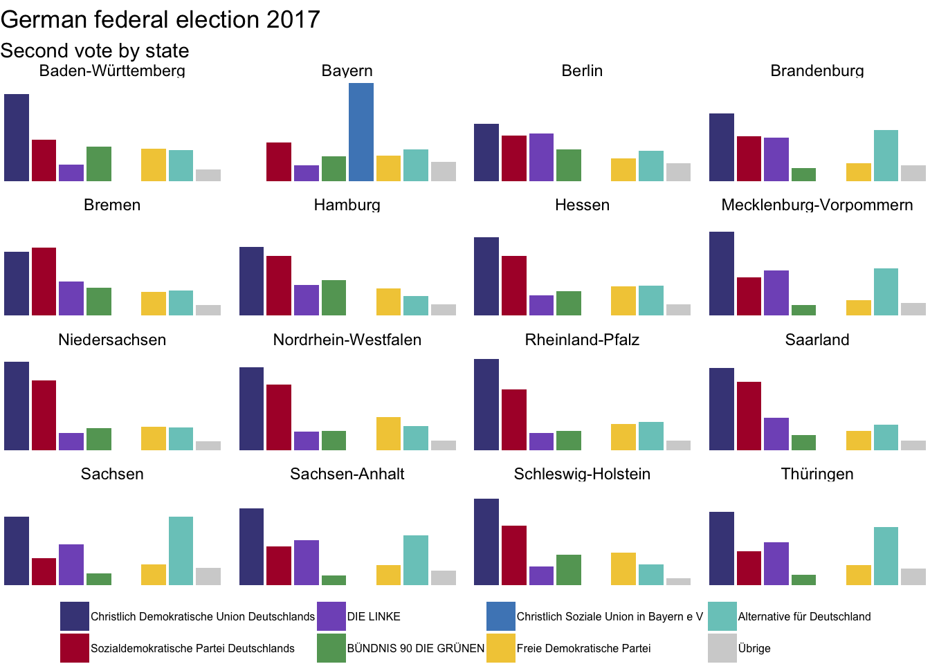

As expected, there is quite a lot of variability. Note that Christlich Soziale Union in Bayern is specific for Bavaria. In the rest of Germany we have Christlich Demokratische Union Deutschlands. Both are relatively similar but it does not mean that they always agree.

A nostalgic look back to the ’30s

We have more data for cities so let’s use it to do a principal component analysis and see if there is a regional homogeneity. Why? Well, I just like principal component analysis. It has to be one of my favorite algorithmic and it generally gives eyes appealing representation of the data.

But wait, 16 Bundesländer total. This isn’t something we can handle with a normal palette chart. Let’s adapt one out of the spectral brewer palette.

# Define the length
colourCount <- length(unique(bundeswahl[states, "Gebiet"]))

# And adapt the 'Set3' palette
getPalette <- colorRampPalette(brewer.pal(9, "Spectral"))

No need to normalize, it’s all in percentage already.

df.pca <- prcomp(bundeswahlPer17[cities, (gueltig+1):ncol(bundeswahlPer17)])
summary(df.pca)
## Importance of components:
##                            PC1    PC2     PC3     PC4     PC5     PC6
## Standard deviation     18.7322 8.0096 5.22733 4.88081 2.60587 1.76243
## Proportion of Variance  0.7363 0.1346 0.05734 0.04999 0.01425 0.00652
## Cumulative Proportion   0.7363 0.8709 0.92823 0.97822 0.99246 0.99898
##                            PC7       PC8
## Standard deviation     0.69653 3.031e-15
## Proportion of Variance 0.00102 0.000e+00
## Cumulative Proportion  1.00000 1.000e+00

Good news, everyone! PC1 and PC2 explain pretty much everything.

# Concatenate all information together
scores <- data.frame(bundeswahlPer17[cities, ], df.pca$x)

# And store the pca plot
pca <- qplot(data = scores, x = PC1, y = PC2, colour = as.factor(gehört.zu),
      size = Wahlberechtigte, alpha = .5) +
  scale_alpha_continuous(guide = FALSE) +
  scale_size_continuous(guide = FALSE) +
  theme_minimal() +
  scale_colour_manual(values = getPalette(colourCount),
                      breaks = bundeswahl[states, "Nr"],
                      labels = bundeswahl[states, "Gebiet"]) +
  labs(title = "German federal election 2017",
       subtitle = "Second vote by city") +
  theme(legend.text = element_text(size = 6), legend.position = "bottom",
        legend.title = element_blank())

Ideally, I’d also like to see what the first two of the principal components actually look like.

# Concatenate relevante information
melted <- melt(df.pca$rotation[, 1:2])

# And store this plot too
PC <- ggplot(data = melted) +
  geom_bar(aes(x = Var1, y = value, fill = Var1), stat = "identity") +
  theme_void() +
  scale_fill_manual(values = bundestagP,
                    name = "Partei",
                    labels = partnames) +
  labs(x = NULL, y = NULL,
       title = "",
       subtitle = "Relative importance in each \nprincipal component") +
  theme(legend.text = element_text(size = 6),
        legend.title = element_blank()) +
  theme(legend.position = "none") +
  facet_wrap(~Var2, ncol = 1)

Here we go.

grid.arrange(pca, PC, ncol = 2, widths = 2:1)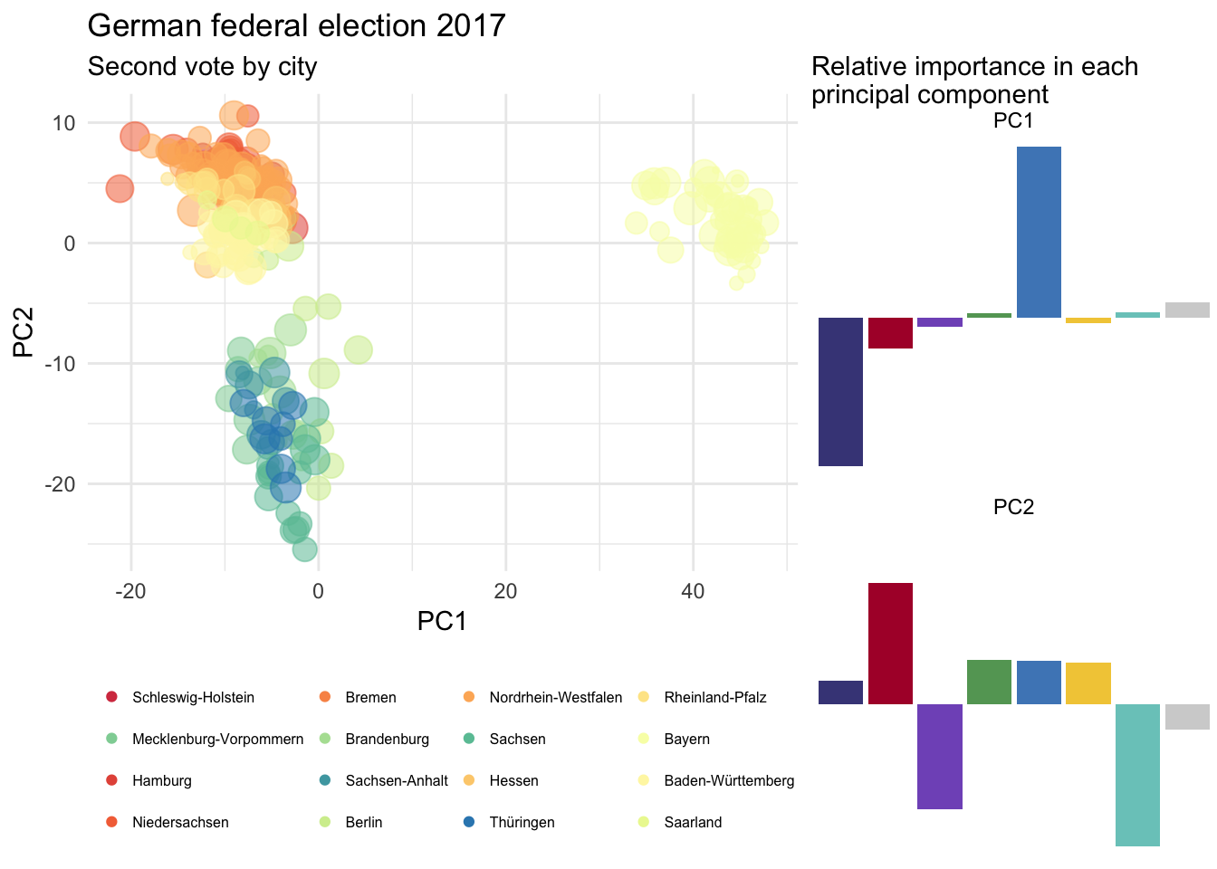

We can compare this with the situation in 2013 if we run the same code using bundeswahl[, vot2old]. I’ve hidden most of it here for the sake of clarity.

## Importance of components:
##                            PC1    PC2     PC3     PC4     PC5     PC6
## Standard deviation     23.6450 8.5221 6.85626 3.72942 1.35207 0.99159
## Proportion of Variance  0.8034 0.1044 0.06755 0.01999 0.00263 0.00141
## Cumulative Proportion   0.8034 0.9078 0.97533 0.99532 0.99794 0.99936
##                            PC7       PC8
## Standard deviation     0.66922 4.501e-15
## Proportion of Variance 0.00064 0.000e+00
## Cumulative Proportion  1.00000 1.000e+00

Roughly the same proportion of the variability explained by PC1 and PC2. And here comes the figure.

grid.arrange(pca13, PC13, ncol = 2, widths = 2:1)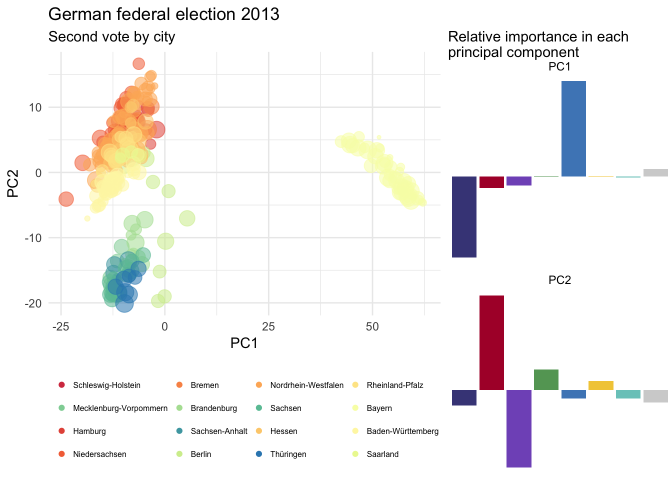

In either case, the PC1 doesn’t contain any valuable information for us. It simply reflect the variability between Christlich Soziale Union in Bayern - specific in Bavaria - and Christlich Demokratische Union Deutschlands in the rest of Germany.

However, everything is swapped in PC2. The Sozialdemokratische Partei Deutschlands and the Alternative für Deutschland are almost inverted. While in 2013 the Sozialdemokratische Partei Deutschlands and DIE LINKE were clearly driving the variability in PC2, in 2017 Alternative für Deutschland is the game changer.

Any doubt about your favorite Bundesländer?

It can be difficult to isolate a specific Bundesland from previous principal component analyses. That is, beside Bavaria. However, we can simply run the code with bundeswahl[states, ]. Again, I’ll hide redundant lines and focus on the most important ones only.

## Importance of components:
##                            PC1    PC2     PC3     PC4    PC5     PC6
## Standard deviation     12.7473 8.9785 4.10249 3.30383 1.7388 0.87088
## Proportion of Variance  0.5912 0.2933 0.06123 0.03971 0.0110 0.00276
## Cumulative Proportion   0.5912 0.8845 0.94573 0.98545 0.9964 0.99921
##                            PC7       PC8
## Standard deviation     0.46691 1.059e-15
## Proportion of Variance 0.00079 0.000e+00
## Cumulative Proportion  1.00000 1.000e+00

I guess it isn’t a surprise now. PC1 and PC2 are sufficient enough, but this time we can identify all Bundesländer.

qplot(data = scoresStates, x = PC1, y = PC2, colour = as.factor(Gebiet),
             size = Wahlberechtigte) +
  scale_alpha_continuous(guide = FALSE) +
  scale_size_continuous(guide = FALSE) +
  theme_minimal() +
  scale_colour_manual(values = getPalette(colourCount),
                      breaks = bundeswahl[states, "Nr"],
                      labels = bundeswahl[states, "Gebiet"]) +
  labs(title = "German federal election 2017",
       subtitle = "Second vote by state") +
  theme(legend.text = element_text(size = 6), legend.position = "bottom",
        legend.title = element_blank()) +
  geom_label_repel(aes(PC1, PC2,
                       label = bundeswahl[states, "Gebiet"]))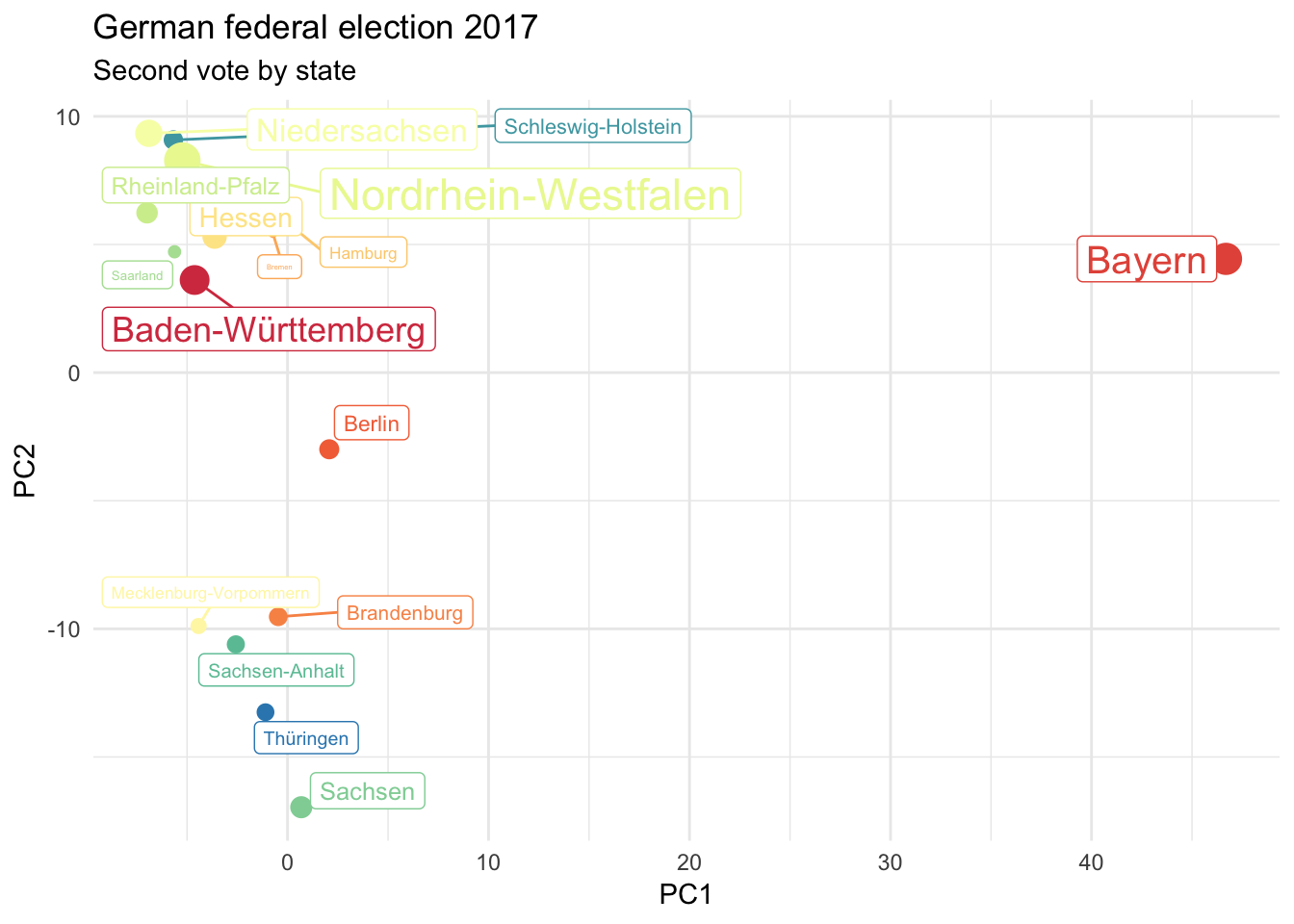

Conclusion

Of course, this doesn’t mean in any way that the Sozialdemokratische Partei Deutschlands or DIE LINKE are responsible for the Alternative für Deutschland breakthrough during this election. But simply that they’ve lost quite a lot of suffrage while the Alternative für Deutschland exploded his previous score - mostly in certain regions. What the PC1 cannot clearly show here is a lost of suffrage for both Christlich Soziale Union in Bayern and Christlich Demokratische Union Deutschlands in 2017 too. This is due to an almost identical lost for both and the overwhelming variability they artificially explain.

Anyway, of interest for Germany here (i) it isn’t by far enough for Martin Schulz to replace Angela Merkel at the head of the country and (ii) which sadly appears divided once again. And once again, Nazis benefit from this. If geography is perhaps not your strong point, you can find a better visual support by the Interaktiv-Team from the Berliner Morgenpost here. They’ve nicely mapped results by party and region.

Is there a good news in all of that misery after all? Yes, I’ve found one =)

# Lower AFD percentage in the whole country is
as.character(bundeswahlPer17[which.min(bundeswahlPer17[, "Alternative.für.Deutschland"]), "Gebiet"])
## [1] "Münster"