Without data you’re just another person with an opinion

The dataset is luckily given to us on a golden plate, with both test and train data included in the titanic package.

# Load the data
train_tit_raw <- titanic_train

The Titanic passengers were divided into three separate classes and anybody who’s watched the movie knows that this, along with the passenger’s sex and fare, plays a big role in survival. In the end Jack dies and Rose survives.

Let’s take a quick look at what we know about these people.

# Greet the data
glimpse(train_tit_raw)
## Rows: 891
## Columns: 12
## $ PassengerId <int> 1, 2, 3, 4, 5, 6, 7, 8, 9, 10, 11, 12, 13, 14, 15, 16, 17…
## $ Survived    <int> 0, 1, 1, 1, 0, 0, 0, 0, 1, 1, 1, 1, 0, 0, 0, 1, 0, 1, 0, …
## $ Pclass      <int> 3, 1, 3, 1, 3, 3, 1, 3, 3, 2, 3, 1, 3, 3, 3, 2, 3, 2, 3, …
## $ Name        <chr> "Braund, Mr. Owen Harris", "Cumings, Mrs. John Bradley (F…
## $ Sex         <chr> "male", "female", "female", "female", "male", "male", "ma…
## $ Age         <dbl> 22, 38, 26, 35, 35, NA, 54, 2, 27, 14, 4, 58, 20, 39, 14,…
## $ SibSp       <int> 1, 1, 0, 1, 0, 0, 0, 3, 0, 1, 1, 0, 0, 1, 0, 0, 4, 0, 1, …
## $ Parch       <int> 0, 0, 0, 0, 0, 0, 0, 1, 2, 0, 1, 0, 0, 5, 0, 0, 1, 0, 0, …
## $ Ticket      <chr> "A/5 21171", "PC 17599", "STON/O2. 3101282", "113803", "3…
## $ Fare        <dbl> 7.2500, 71.2833, 7.9250, 53.1000, 8.0500, 8.4583, 51.8625…
## $ Cabin       <chr> "", "C85", "", "C123", "", "", "E46", "", "", "", "G6", "…
## $ Embarked    <chr> "S", "C", "S", "S", "S", "Q", "S", "S", "S", "C", "S", "S…

• PassengerID has to be a random unique identifier, and has no impact on the outcome variable. We can happily ignore it for this work.
• Survived variable is our outcome or dependent variable. It is a binary nominal datatype of 1 for survived and 0 for did not survive.
• Pclass is an ordinal datatype for the ticket class indicating passenger socio-economic status, 1 = upper, 2 = middle, and 3 = lower.
• Name is a nominal datatype. It’s relatively useless as such, but can be used in feature engineering to derive gender and precise title.
• Sex is, well, quite straightforward right?
• Age is… Oh come on, I shouldn’t have to explain you all this really.
• SibSp represents number of related siblings/spouse aboard and;
• Parch the number of related parents/children aboard. Could be used to determine how many relatives were present on board.
• Ticket is useless here. It might include information about class or fare but cannot be decoded. This has to be excluded too.
• Fare is a continuous quantitative datatype. The price charged to transport the passenger.
• Cabin could be used to determine approximate position on ship during the disaster (iceberg was hit at 11:40pm ship’s time).
• Embarked is a nominal datatype indicating the port of embarkation.

Using this we’d like to predict which passengers survived the tragedy and what are the most important variables.

Prepare data for consumption

Most of the work has been done already and there is no need for hardcore data wrangling. The package provides easily manageable data. Nevertheless, we can do some data cleaning to identify aberrant or missing data points and potential information we can derive from what is included here.

First let’s look at a NA’s X-ray 1. I call it like this because it returns something very similar to an X-ray, only it highlights missing values.

# Heatmap all NAs
train_tit_raw %>%
  is.na %>%
  melt %>%
  # plot a visual take on the missing values
  ggplot(aes(x = Var2, y = Var1)) +
  geom_raster(aes(fill = value)) +
  scale_fill_brewer(palette = "Greys") +
  theme_minimal() +
  theme(axis.text.x = element_text(angle = 45, vjust = .5),
        panel.grid.minor=element_blank(),
        panel.grid.major=element_blank(),
        axis.text.y = element_blank()) +
  theme(legend.position = "none") +
  labs(x = NULL, y = "PassengerID",
       title = "NA's X-ray",
       subtitle = "NA's are displayed black",
       caption = "source: Titanic passenger survival data set")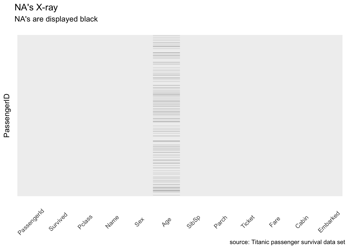

Figure 1: X-ray highlighting missing values.

Okay, so there are some NA values in the age. This could be bad as some algorithms don’t know how-to handle null values. I propose we impute Age simply using the median for now.

There are many, too many, null values in Ticket as well. But I said earlier this variable will be dropped anyway as we cannot decode it.

train_tit <- train_tit_raw %>% 
  mutate(Age = replace_na(Age, median(Age, na.rm = TRUE))) %>% 
  # and remove PassengerId, Ticket, and Cabin
  select(-PassengerId, -Ticket, -Cabin)

More predictors do not make a better model

But selecting the right variables helps, quite a lot. Many independent features that each correlate well with the class will make the learning easier and of course, if the class is a very complex function of the features, you may not be able to learn it at all. Doing machine learning often implies spending quite a long time getting the raw data in a form that allows best to learn from it. It can also be one of the most interesting parts and has been described as the most important factor in determining the success or failure of your predictive model.

Three quick examples to help illustrate this.

First guess: the passenger’s class matters.

train_tit %>% 
  group_by(Pclass) %>%
  summarise(died = sum(Survived == 0),
            total = n(),
            freq = died/total)
## # A tibble: 3 x 4
##   Pclass  died total  freq
## *  <int> <int> <int> <dbl>
## 1      1    80   216 0.370
## 2      2    97   184 0.527
## 3      3   372   491 0.758

Bingo… Okay, okay, this was clear already. But helps us set a baseline.

Let’s save this as an histogram for a visualization down the road 2.

pClass <- train_tit %>% 
  mutate(Pclass = factor(case_when(Pclass == 1 ~ "First",
                                   Pclass == 2 ~ "Second",
                                   Pclass == 3 ~ "Third"),
                         # let's scale x as we know the rates already
                         levels = c("Third", "Second", "First"))) %>% 
  group_by(Pclass) %>%
  summarise(died = sum(Survived == 0),
            total = n(),
            freq = died/total) %>% 
  ggplot(aes(x = Pclass, y = freq, fill = as.factor(Pclass))) +
  geom_bar(stat = "identity", alpha = .9, position = position_dodge()) +
  theme_minimal() +
  scale_fill_brewer(palette = "RdYlBu") +
  theme(legend.position="none") +
  labs(x = NULL, y = "Death rate",
       title = "Death rate among passengers",
       subtitle = "Organized from the highest to the lowest death rate",
       caption = "")

Second one: the passenger’s title too. Remember this can be extracted from the column Name.

train_tit %>% 
  mutate(Title = case_when(grepl("Miss.", Name) ~ "Miss.",
                           grepl("Mrs.", Name) ~ "Mrs.",
                           grepl("Mr.", Name) ~ "Mr.",
                           grepl("Master.", Name) ~ "Master.",
                           # the rest represents ~2%
                           TRUE ~ as.character("Others"))) %>% 
  group_by(Title) %>%
  summarise(died = sum(Survived == 0),
            total = n(),
            freq = died/total)
## # A tibble: 5 x 4
##   Title    died total  freq
## * <chr>   <int> <int> <dbl>
## 1 Master.    17    40 0.425
## 2 Miss.      55   182 0.302
## 3 Mr.       436   518 0.842
## 4 Mrs.       26   127 0.205
## 5 Others     15    24 0.625

Here we go.

I’m a little unsure about the meaning of Master here. This isn’t an academic title as it seems reserved to very young male children. Whatever is special about them, at least we can say they’ve definitively mastered the art of survival at sea.

Okay, let’s save this one as an histogram too 2.

title <- train_tit %>% 
  mutate(Title = factor(case_when(grepl("Miss.", Name) ~ "Miss.",
                                  grepl("Mrs.", Name) ~ "Mrs.",
                                  grepl("Mr.", Name) ~ "Mr.",
                                  grepl("Master.", Name) ~ "Master.",
                                  # the rest represents ~2%
                                  TRUE ~ as.character("Others")),
                        # let's scale x as we know the rates alread
                        levels = c("Mr.", "Others", "Master.", "Miss.", "Mrs."))) %>% 
  group_by(Title) %>%
  summarise(died = sum(Survived == 0),
            total = n(),
            freq = died/total) %>% 
  ggplot(aes(x = Title, y = freq, fill = Title)) +
  geom_bar(stat = "identity", alpha = .9, position = position_dodge()) +
  theme_minimal() +
  scale_fill_brewer(palette = "RdYlBu") +
  theme(legend.position="none") +
  labs(x = NULL, y = "",
       title = "",
       subtitle = "",
       caption = "")

Last guess: who had family on board.

train_tit %>% 
  mutate(Family = case_when(SibSp == 0 & Parch == 0 ~ "Alone",
                            SibSp == 1 & Parch == 0 ~ "Couple",
                            SibSp == 0 & Parch >= 1 ~ "Parents",
                            SibSp >= 2 & Parch == 0 ~ "Siblings",
                            SibSp >= 1 & Parch >= 1 ~ "Family")) %>% 
  group_by(Family) %>%
  summarise(died = sum(Survived == 0),
            total = n(),
            freq = died/total)
## # A tibble: 5 x 4
##   Family    died total  freq
## * <chr>    <int> <int> <dbl>
## 1 Alone      374   537 0.696
## 2 Couple      59   123 0.480
## 3 Family      80   142 0.563
## 4 Parents     24    71 0.338
## 5 Siblings    12    18 0.667

This looks interesting too. Being on your own or with siblings only was the worse case. Lonely travelers were predominantly male. Having your family on board really increased chances of at least some surviving the disaster probably because these families were able to “save women and children first”. Being a couple certainly helped you to save at least your wife and travelling as a parent with children was the best way to find a seat in a lifeboat.

We should save this as well 2.

family <- train_tit %>% 
  mutate(Family = factor(case_when(SibSp == 0 & Parch == 0 ~ "Alone",
                                   SibSp == 1 & Parch == 0 ~ "Couple",
                                   SibSp == 0 & Parch >= 1 ~ "Parents",
                                   SibSp >= 2 & Parch == 0 ~ "Siblings",
                                   SibSp >= 1 & Parch >= 1 ~ "Family"),
                         # let's scale x as we know the rates already
                         levels = c("Alone", "Siblings", "Family", "Couple", "Parents"))) %>% 
  group_by(Family) %>%
  summarise(died = sum(Survived == 0),
            total = n(),
            freq = died/total) %>% 
  ggplot(aes(x = Family, y = freq, fill = Family)) +
  geom_bar(stat = "identity", alpha = .9, position = position_dodge()) +
  theme_minimal() +
  scale_fill_brewer(palette = "RdYlBu") +
  theme(legend.position="none") +
  labs(x = NULL, y = "",
       title = "",
       subtitle = "",
       caption = "source: Titanic passenger survival data set")

Finally, we can quickly organize this into a layout.

grid.arrange(pClass, title, family, layout_matrix = rbind(c(1 ,2, 2), c(1, 3, 3)))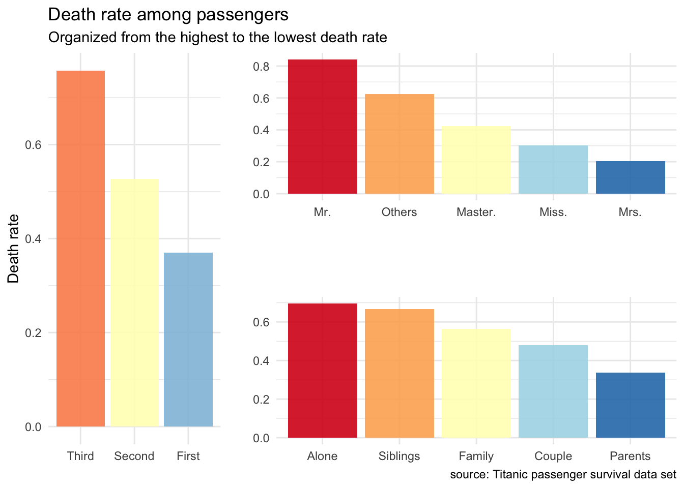

Figure 2: Death rate among passengers.

Looking at all this, being a married woman, travelling first class and with some members of your family, particularly children gave you the best survival chance. But is this all we can say?

How to beat the odds

Binary events create an interesting dynamic, because we know statistically when we flip a coin that a random guess should achieve a 50% accuracy rate - in other words, you have a 50-50 chance of guessing correct - without creating one single algorithm or writing one single line of code. Therefore 50% would be the worst model performance (and actually in this particular case, extremely difficult to beat even with some heavy machine learning).

But wait a minute… We already can do better here. Much better and with just one line of code.

train_tit %>% 
  summarise(died = sum(Survived == 0),
            total = n(),
            freq = died/total)
##   died total      freq
## 1  549   891 0.6161616

We have 891 people in this training dataset and 549 of them died. If we just predict the most frequent occurrence, simply guessing that all of them died, then we would be right 61.62% of the time. We can see 61.62% as bad model performance. Anything lower than that, I can just predict using the most frequent occurrence.

This sets the baseline and of course, is where the challenge really starts.

By the way, we have seen this 61.62% in our three guesses before, although slightly disguised. First guess, passenger’s class for example (0.3703704 * 216 + 0.5271739 * 184 + 0.7576375 * 491) / 891 = 0.6162. Same for the two others of course, do the math and you will see it for yourself.

What if we’d like to get a rough estimate of the difficulty here? Remember that many independent features that each correlate well with the class will make the learning easier. We can plot a heatmap including all you predictors and check this quickly.

Let’s prepare train_tit_coded for the heatmap as we need to code these character variables as numerical factors.

train_tit_coded <- train_tit %>% 
  mutate(Title = case_when(grepl("Miss.", Name) ~ "Miss.",
                           grepl("Mrs.", Name) ~ "Mrs.",
                           grepl("Mr.", Name) ~ "Mr.",
                           grepl("Master.", Name) ~ "Master.",
                           # the rest represents ~2%
                           TRUE ~ as.character("Others")),
         Family = case_when(SibSp == 0 & Parch == 0 ~ "Alone",
                            SibSp == 1 & Parch == 0 ~ "Couple",
                            SibSp == 0 & Parch >= 1 ~ "Parents",
                            SibSp >= 2 & Parch == 0 ~ "Siblings",
                            SibSp >= 1 & Parch >= 1 ~ "Family")) %>% 
  select(-Name) %>% 
  mutate_if(is.character, as.factor) %>% 
  mutate_if(is.factor, as.numeric)

Now we can quickly plot a matrix 3 to classify parameters and determine correlation with the target (i.e., Survival). This matrix can be ordered using a hierarchical clustering to facilitate the identification of hidden structures and patterns. Also we can cross out the less significant values.

# Calculate correlation matrix
corr.matrix <- train_tit_coded %>%
  keep(is.numeric) %>%
  cor(method = c("pearson"))

# Significance test
cor.mtest <- train_tit_coded %>%
  keep(is.numeric) %>%
  cor.mtest(conf.level = .95)

# Plot correlation matrix
corrplot(corr.matrix, method = "square", order = "hclust", 
         addrect = 4, p.mat = cor.mtest$p, sig.level = .2,
         col = brewer.pal(n = 10, name = "RdYlBu"), tl.col = "black")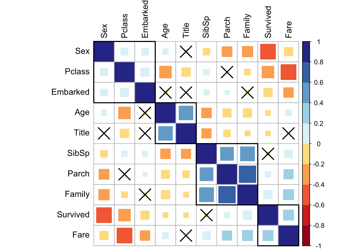

Figure 3: Correlation matrix.

The most important here is probably the relation among SibSp, Parch, and Family which is quite obvious. Age and Title seem to correlate and I bet this is at least partially due to our young Masters.

Interestingly, there is some relation in between Sex, Pclass, and Embarked. But overall, it looks like we’ve a couple of features that, even if with some dependency, each correlate well with the Survival. This will certainly allow us to learn something more with a model.

Build the model

So can we do better now, combining all these predictors and giving the machine a chance to do its magic so as to learn how to predict this outcome? To answer this question let’s simply start with a decision tree model. We are simply asking questions after questions and segment our target response placing the survivors and deceased into homogeneous subgroups.

But first, we will need to partition the data into training and testing groups. This is something I’ve already been explaining in my previous post when classifying mushrooms as edible or poisonous.

First let’s create the titanic_tbl.

titanic_tbl <- train_tit %>% 
  mutate(Title = case_when(grepl("Miss.", Name) ~ "Miss.",
                           grepl("Mrs.", Name) ~ "Mrs.",
                           grepl("Mr.", Name) ~ "Mr.",
                           grepl("Master.", Name) ~ "Master.",
                           # the rest represents ~2%
                           TRUE ~ as.character("Others")),
         Family = case_when(SibSp == 0 & Parch == 0 ~ "Alone",
                            SibSp == 1 & Parch == 0 ~ "Couple",
                            SibSp == 0 & Parch >= 1 ~ "Parents",
                            SibSp >= 2 & Parch == 0 ~ "Siblings",
                            SibSp >= 1 & Parch >= 1 ~ "Family")) %>% 
  select(-Name) %>% 
  mutate_if(is.character, as.factor) %>% 
  select(Survived, everything())

Then set some seeds for reproducibility and split it.

set.seed(123)

# Split test/training sets
train_test_split <- initial_split(titanic_tbl, prop = 0.8)

# Quick sanity check
train_test_split
## <Training/Validation/Total>
## <713/178/891>

Training and testing sets can be retrieved using training() and testing() functions.

# Retrieve train
train_tit_tbl <- training(train_test_split)

# And test sets
test_tit_tbl <- testing(train_test_split) %>% 
  mutate(Survived = as.factor(case_when(Survived == 0 ~ "No",
                                        Survived == 1 ~ "Yes")))

And here comes the decision tree 4 that we can render with fancyRpartPlot from rpart.plot.

# Build the model tree
model_tree <- rpart(Survived ~ ., method = "class", data = train_tit_tbl)

# Draw a decision tree
fancyRpartPlot(model_tree, sub = "")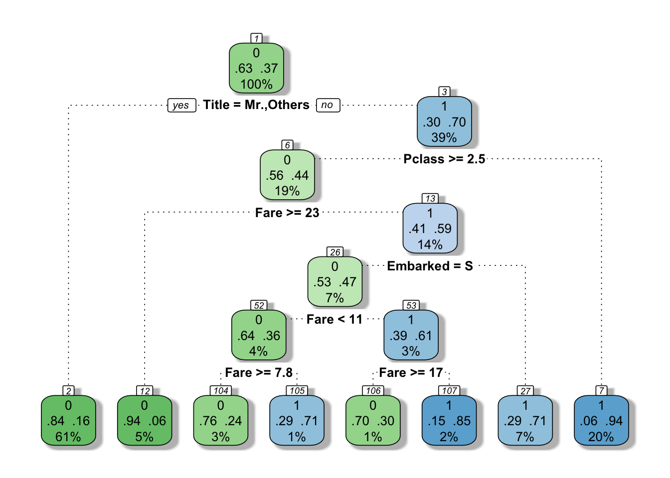

Figure 4: Fancy decision tree

This decision tree goes deeper than the initial guesses. It’s a bit like a “Guess who” game. First question asked here is is your passenger a Mr.? that resonates well with the famous “save women and children first”. Then if yes, did your passenger pay a fare inferior to 26?; or if no, was your passenger travelling third class?, etc.

But what about making a real prediction using the test set now. Did all this help improve the accuracy?

# Let the model do its magic
fitted_results_tree <- predict(model_tree, test_tit_tbl, type = "class")
test_tit_tbl$predicted_tree <- as.factor(ifelse(fitted_results_tree == 1, "Yes", "No"))

# Create confusion matrix
confMatrix_tree <- caret::confusionMatrix(data = test_tit_tbl$predicted_tree,
                                          reference = test_tit_tbl$Survived,
                                          positive = "Yes")

confMatrix_tree$table
##           Reference
## Prediction No Yes
##        No  95  31
##        Yes  6  46
confMatrix_tree$overall[1]
##  Accuracy 
## 0.7921348

Yes, 79.21%. We nailed it down with an extra 17.6% accuracy.

Can we beat this?

At least we should try. Decision trees will quickly overfit to the data - when a model performs well on a training set, but does worse on unseen data - because all passenger’s story are different and the rule defined here may not generalize well to unknown passengers.

How to avoid this?

Simply let the trees vote. Yes, vote. The prediction works in a similar way: in a random forest model each tree make its classification decisions based on different variables, except that after all trees made their decisions they discuss who’s right.

# Build the random forest
model_rf <- randomForest(Survived ~ ., importance = TRUE, ntree = 2000, data = train_tit_tbl)

I’ve happily set 2000 trees here. Whoever’s seen another movie (or much better, read the books) knows that trees can argue for quite a long time before taking any decisions. However, this dataset doesn’t contain that many observations and 2000 isn’t really going to slow us down.

# Let the model do its magic
fitted_results_rf <- predict(model_rf, test_tit_tbl, type = "class")
test_tit_tbl$predicted_rf <- as.factor(ifelse(fitted_results_rf > .5, "Yes", "No"))

# Confusion matrix
confMatrix_rf <- caret::confusionMatrix(data = test_tit_tbl$predicted_rf,
                                        reference = test_tit_tbl$Survived,
                                        positive = "Yes")

confMatrix_rf$table
##           Reference
## Prediction No Yes
##        No  92  32
##        Yes  9  45
confMatrix_rf$overall[1]
##  Accuracy 
## 0.7696629

Awesome! 76.97%. We improved the decision tree by another -2.25% accuracy.

We want to be approximately right, rather than exactly wrong

Although 76.97% isn’t probably the best we can achieve we’ve come a long way already, from the 61.62% baseline to the 76.97% accuracy of the random forest. There is no no free lunch theorem of machine learning, no super algorithm, that works best in all situations, for all datasets. We simply tried different implementations of a decision tree, which is the easiest concept to learn and understand. There are other flavors we didn’t talk about yet, nor did we tune our models at all here.

Interestingly, the Title variable we derived from the Name was used in the first question asked by the decision trees. The question was is your passenger a Mr.? and not is your passenger a male?. Young males, particularly children, had better survival chances than married adults. This is a nice example of how feature engineering can help extract better variables and is were most of the work goes. There is certainly more we can do here and I’m sure the accuracy can be improved, but I’m afraid we will never be able to save Jack.