How to retrieve series from the WHO

# Retrieve series, codes, and descriptions
codes <- get_codes()
str(codes)
## tibble [3,316 × 3] (S3: tbl_df/tbl/data.frame)
##  $ label  : chr [1:3316] "MDG_0000000001" "MDG_0000000003" "MDG_0000000005" "MDG_0000000006" ...
##  $ display: chr [1:3316] "Infant mortality rate (probability of dying between birth and age 1 per 1000 live births)" "Adolescent birth rate (per 1000 women aged 15-19 years)" "Contraceptive prevalence (%)" "Unmet need for family planning (%)" ...
##  $ url    : chr [1:3316] "https://www.who.int/data/gho/indicator-metadata-registry/imr-details/1" "https://www.who.int/data/gho/indicator-metadata-registry/imr-details/4669" "https://www.who.int/data/gho/indicator-metadata-registry/imr-details/5" "https://www.who.int/data/gho/indicator-metadata-registry/imr-details/6" ...

So far they are 3316 datasets available, which are all easily retrieved through the get_data function. But first we need to pick-up series of interest. Let’s say we want to analyze breast cancer data and search for them among the series with a regular expression.

# Search for series about breast cancer
breastCancer <- codes[grep("[Bb]reast [Cc]ancer", codes$display),]
breastCancer$display
## [1] "Age-standardized DALYs, breast cancer, per 100,000"                                                          
## [2] "Age-standardized death rates, breast cancer, per 100,000"                                                    
## [3] "General availability of breast cancer screening (by palpation or mammogram) at the primary health care level"
## [4] "Existence of national screening program for breast cancer"                                                   
## [5] "Age-standardized DALYs, breast cancer, per 100,000"                                                          
## [6] "Age-standardized death rates, breast cancer, per 100,000"

So we have age-standardized disability-adjusted life years (DALYs), age-standardized death rates, and general availability of breast cancer screening at the primary health care level there. Certainly enough to run some test analyses. Okay let’s first fetch the data through the get_data function.

# Retrieve the dataframes from the internet
DALYs <- get_data(breastCancer$label[1])
deathRates <- get_data(breastCancer$label[2])
cancerScreening <- get_data(breastCancer$label[3])

Interlude

Maybe you are relatively new to R. If you recently installed it on your computer and didn’t have time to explore the CRAN you might want to run the following code to ensure you have all the required packages installed. All of them are very useful anyway: you won’t regret it!

# Required packages from CRAN
.pkgs = c("dplyr", "ggplot2", "RColorBrewer")

# Install required packages from CRAN (if not)
.inst <- .pkgs %in% installed.packages()
if(length(.pkgs[!.inst]) > 0) install.packages(.pkgs[!.inst])

After that, be sure to load them all.

# Load required packages
library(dplyr)
library(ggplot2)
library(RColorBrewer)

Let’s create our dataframe

After loading the data, we surely want to combine our three dataframes together. Male breast cancers are relatively rare, about 1% of all breast cancers only and are usually diagnosed at a more advanced stage. Therefore, I choose to filter them out and to return here the female breast cancers only.

# Filter, combine and group together
df <- data.frame(deathRates %>%
                   filter(sex == "Female") %>%
                   group_by(year, country) %>%
                   summarise(region, value),
                 DALYs %>%
                   filter(sex == "Female") %>%
                   group_by(year, country) %>%
                   summarise(value),
                 cancerScreening %>%
                   filter(country %in% DALYs$country) %>%
                   group_by(year, country) %>%
                   summarise(value))

There is some redundancy in the country and year columns that needs to be removed. A simple way to do that is to use a regular expression again. Once you’ve selected the redundant columns, it becomes easy to clean the dataframe.

# Search and remove redondancy
sel.cl <- grep("*[yr].[12]", colnames(df), invert = TRUE)
df <- df[,sel.cl]

Finally, let’s quickly adjust the column’s names of our dataframe.

# Rename columns
colnames(df) <- c("year", "country", "region", "deathRates", "DALYs", "cancerScreening")
df[1:10,]
##    year             country                region deathRates DALYs
## 1  2004         Afghanistan Eastern Mediterranean       29.6   506
## 2  2004             Albania                Europe       28.7   384
## 3  2004             Algeria                Africa       17.5   212
## 4  2004             Andorra                Europe       18.4   267
## 5  2004              Angola                Africa       34.5   410
## 6  2004 Antigua and Barbuda              Americas       37.7   549
## 7  2004           Argentina              Americas       25.8   316
## 8  2004             Armenia                Europe       38.6   552
## 9  2004           Australia       Western Pacific       20.3   337
## 10 2004             Austria                Europe       20.1   259
##     cancerScreening
## 1               Yes
## 2               Yes
## 3               Yes
## 4               Yes
## 5  No data received
## 6               Yes
## 7               Yes
## 8               Yes
## 9               Yes
## 10              Yes

Now what?

Well, how about plotting the data now?

ggplot(df, aes(x = deathRates, y = DALYs, color = region, shape = cancerScreening)) +
  geom_point() +
  theme_minimal() +
  ggtitle("") +
  xlab("Death rates (per 100,000)") +
  ylab("DALYs (per 100,000)") +
  scale_shape_manual(values = c(1:5), name = "Screening") +
  scale_color_brewer(palette = "Set1", name = "Region") +
  theme(legend.position = "bottom") +
  theme(legend.title = element_blank())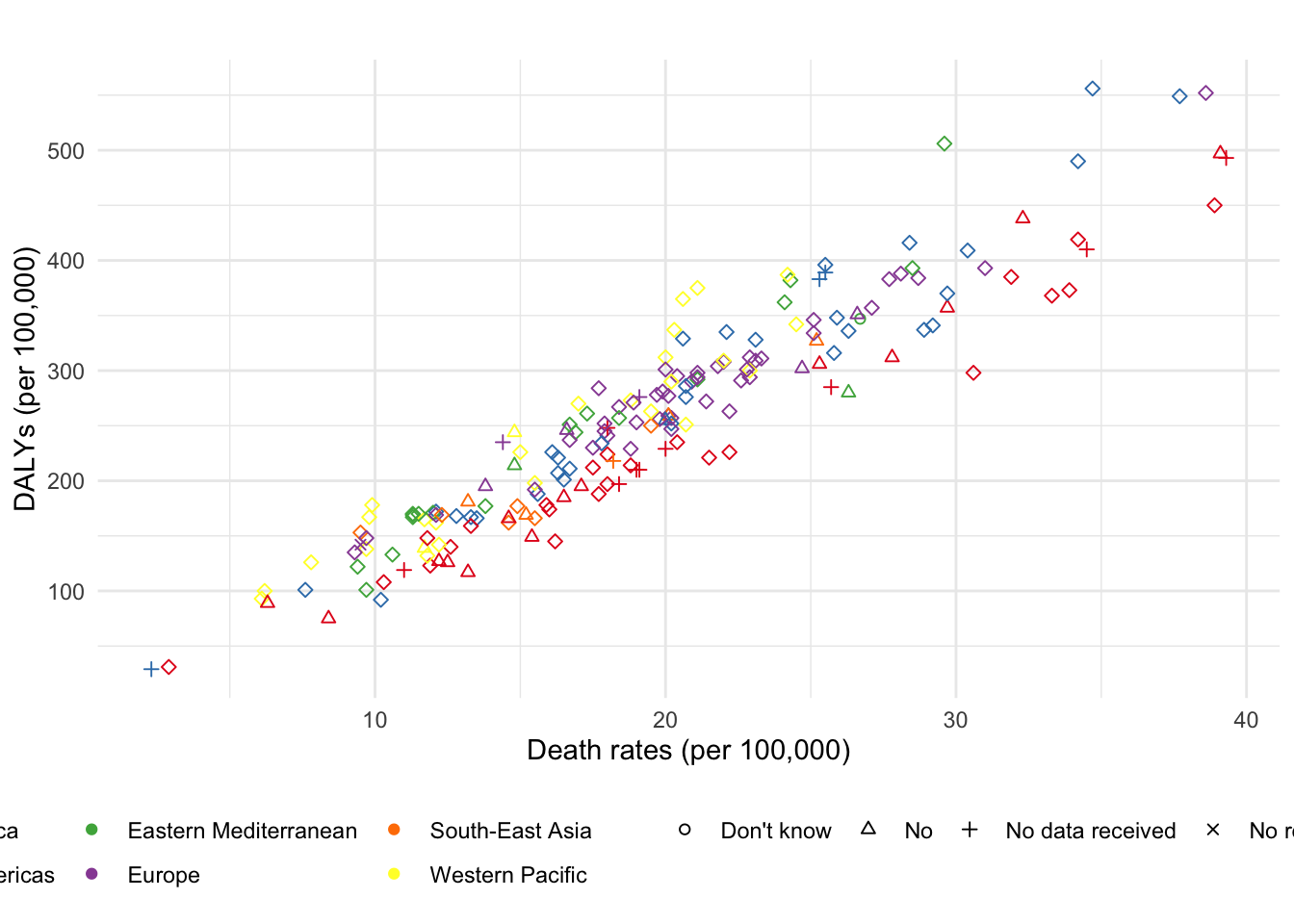

Figure 1: A fancy scatterplot.

Two assumptions were made in figure 1: death rates and DALYs were published in 2004, whereas the data about the availability of screening is from 2013. We can reasonably assume that countries with no screening at the primary health care level in 2013 didn’t have screening back in 2004 either. But there is no way to be sure that countries organizing screening for breast cancer nowadays were already doing it in 2004. Additionally, there is no data about patient’s sex in the breast cancer screening data set. But one can assume that it was a least available to female patients, since they are usually the only population targeted by routine screening for breast cancer.